Statistical Analyses of Victims 1-3 Treatment to Predict Team Versus Solo Serial Killers
Nikki Igo, MS-IV., Oklahoma State University Center for Health Sciences
John Harden., Oklahoma State University, Educational Psychology
Research, Evaluation, Measurement, and Statistics (REMS) PhD Student
Jason Beaman D.O., M.S., M.P.H., FAPA., Assistant Clinical Professor.,
Chair, Department of Psychiatry and Behavioral Sciences., Oklahoma State University Center for Health Sciences
Introduction
The act of committing homicide is difficult to fathom. Even more difficult to fathom is repeating the act of homicide to attain the title of ‘serial killer’. Moreover, when you factor in the existence of serial killer teams, the topic becomes almost inconceivable. The fact that there are multiple victims to study within a single team or subject’s profile has allowed the topic to be persistently popular among researchers 1. While there is ample research available on serial homicide, one subtopic that has received comparatively little attention is the analysis of the behavior of serial killer teams and comparison with solo killers 2. This study aims to explore the data available through the Radford/FGCU Serial Killer Database and identify noteworthy characteristics of team killers and their behaviors that are not displayed as prominently by solo serialists. Identification of these characteristics was done through a logistic regression analysis of the data for the first three victims of both serial killer teams and solo serialists. The results of this study could aid in determination of whether the subjects being pursued in active investigations are acting as teams or individually. It is also the goal of this study to draw attention to a research area in need of further investigation and identify areas for future discussion and exploration.
Methods
The Radford/Florida Gulf Coast University Serial Killer Database used in analyses was accessed on 5/16/2019 and included 503 variables with 2,377 serial killer observations. Of those, 1,285 contained three or more victims. Missing data included blank values for Serial Killer Team’s variables Serial Killer DOB, Serial Killer Sex, Serial Killer Sexual Preference, Serial
Killer Race, due to multiple serial killers involved in the act, so these variables were not included in analysis.
Victim #[...] Treatment variables contained all known treatments for each victim, such as whether they were killed quickly, stalked, and/or raped. As a result, the variables were converted into a series of dummy variables, where each Victim Treatment parameter was given its own variable. This resulted in 16 dummy variables of Victim Treatment for each victim. This approach was similarly taken with Victim #[…] Method of Kill variables and Victim #[…] Weapon variables, resulting in 16 and seven additional dummy variables per victim, respectively. The highest total victim count for all Serial Killers was 56, meaning a total of 2,184 dummy variables were created (56 victims * (16 Victim Treatments + 16 Methods of Kill + 7 Weapons), with the intent to use the expanded data set in future analyses.
The research question involved analyzing only whether the victim treatment, weapon used, and method of killing of the first three victims could predict whether the act was committed by individuals or teams. They hypothesis being tested is that treatment of the first three victims, how the victims were killed, and the weapon(s) used may be different for individual and team killers.
Each victim treatment dummy variable was averaged for the first three victims of each killer or team of killers and variables were created that contained these averages. The weapon and then the method of killer dummy variables were averaged and recorded in new variables in the same manner. Serial killer teams were coded as “1” and individuals were coded as “0” in a single variable. Of the 1,285 instances of teams and individuals with three or more kills, 127 instances were recorded as teams.
Forward stepwise binary logistic regression was conducted using all of the three victim averages for victim treatment, weapon, and method of kill dummy variables for a subset of data that included all 127 team killers and the first 127 individuals listed in the data. This subset was created to reduce oversampling of individual killers compared to team killers. Initial analyses with Dependent Variable as “0” for individual and “1” for Teams with 3-victim-averages for 16 Victim Treatment, 16 Methods of Kill, and 7 Weapons. Independent Variables (IVs) that failed to produce statistical analysis software output due to limited instances of certain included variables were removed in subsequent analysis. Forward stepwise binary logistic regression was again conducted, with the majority of IVs presenting non-significance (p> 0.05). The non-significant IVs were omitted from further analysis.
Significant Victim Treatment variables included the three-victim-averages for Quick, Stalk, and Rape, the three-victim-average for Gun Death weapon variable, and no Method of Kill variables. There was some concern about potential multicollinearity between Method of Kill IVs and the Weapon IVs, but this was not an issue as no Method of Kill IVs were used in final analyses. Significant values for this initial analysis are reported in the Results section. Eight additional forward stepwise binary logistic regression analyses were conducted with the remaining data in such a way that no individual serial killer instance was repeated, while all 127 serial killer teams were included in each analysis. The average number of individual killers for each analysis was 128.67 (with three models containing 128 individual killer instances and six models containing 129).
Three additional logistic regressions were conducted on 85 random team serial killers and 85 individuals, with the possibility of any instance being in any, all, or none of the analyses, for data validation. Categorical Principal Component Analysis (CatPCA) was conducted on the same three groupings of 85 random individuals and teams as additional data validation, using the significant IVs from the logistic models (the 3-victim-average variables for Quick, Stalk, Rape, and Gun Death) and the DV binary variable Teams/Individual Killer. CatPCA was chosen over other dimension reduction techniques due to the binary variable identifying individuals or teams.
A supplementary analysis was conducted to examine whether three victims’ data per instance was necessary to create a prediction model: additional logistic regression analyses were conducted on a single group of 127 individuals and 127 teams using the victim treatment, weapon, and method of kill dummy variables first for a single victim, then for the first two victims, and then for all three victims.
Results
By ensuring near-equal or equal counts of individual (either 128 or 129 instances for initial models and 85 for validations models) and team (127 for all initial models and 85 for validation models) killers, and with the use of post-hoc Nagelkerke R Square values from each model, the models had power equal to one for all models, calculated with G*Power 3.1.9.4. The greatest correlation between any variables or constants in all models was -0.575 (3-victim-average for Gun Death with the Constant), indicating an absence of multicollinearity.
Initial Models
Nine binary logistic regression analyses were conducted using SPSS Statistics 27 with samples of 127 serial killer teams and between 128 and 129 individual serial killer instances (three models with 128 and six with 129), in order to include all individual killers in such a way they were not repeated (9 groups of individuals) against the total sample of team killers (total of 127 in a single group used in each analysis). The differences in sample sizes for individuals was to ensure all individual serial killer instances were included in an analysis. Variables for the average of the first three victims for each instance that were killed quickly, stalked, raped, and killed by gun were significant (p<.05) in all nine models, which were the only variables used in analysis. These variables were created from averaging the respective dummy variables, resulting in categorical variables with four values, 0, 0.333, 0.667, and 1. All assumptions for binary logistic regression were met.
The worst performing of the nine models correctly predicted individuals committed the killings 79.8% of the time, and correctly predicted teams were responsible for committing the killings 92.1% of the time. The best performing model correctly predicted individuals 89.1% of the time and teams 92.1% of the time. The ranges from all nine models was 79.1-89.1% correct prediction for individuals and 92.1-96.1% for teams, with means of correct prediction for individuals and teams as 83.8% and 92.5%, respectively.
The Classification Tables for the initial nine models can be seen in Table 1.
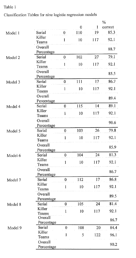
The Nagelkerke R Square for the worst performing model was 0.656, meaning an approximation for the variance explained by the model was 65.6%. The Nagelkerke R Square for the best performing model was 0.766, or an approximation of 76.6% variance accounted for. The mean Nagelkerke R Square was 0.702, or a 70.2% approximation of variance accounted for.
The average binary logistic regression model for the nine models was found to be Serial Killer Team = 0.929[Constant] + -3.510*Quick Kill + -3.850*Stalking + -3.360*Rape + 1.841*Gun Death, where positive values indicated the act was predicted to be an instance of Serial Killer Teams and negative values indicative of Individual Serial Killers. The range of beta weights for the independent variables and constants were -3.494 to -2.707 for Quick Kill, -4.547 to -3.548 for Stalking, -3.881 to -2.742 for Rape, 1.186 to 2.495 for Gun Death, and 0.614 to 1.245 for the constant. These results, as all lows and highs for all independent variables were of the same sign, support the finding that Serial Killer Teams are more likely to kill by gun and less likely to kill quickly, stalk, or rape, and the opposite was found for Individual Serial Killers, across all models.
The regression formula including the ranges of each model would be: Serial Killer Teams (1 or 0) = 0.614 to 1.245 [the Constant] + -3.494 to -2.707 * [Quick Kill value] + -4.547 to -3.548 * [Stalking value] + -3.881 to -2.742 * [Rape value] + 1.186 to 2.495 * [Gun Death value]. Each serial killer instance was applied to the models to predict whether the incident was perpetrated by individuals or teams of killers. The individual binary logistic regression model output for the nine models can be seen in Table 2.
Table 2
Model summaries for nine initial logistic regression models
|
B |
S.E. |
Wald |
df |
Sig. |
Exp(B) |
EXP(B) 95% C.I. Lower |
EXP(B) 95% C.I. Upper |
| Group 1 |
| 3VicAve_Quick |
-3.15 |
0.56 |
31.65 |
1 |
0.000 |
0.043 |
0.014 |
0.128 |
| 3VicAve_Stalk |
-3.62 |
0.77 |
21.9 |
1 |
0.000 |
0.027 |
0.006 |
0.122 |
| 3VicAve_Rape |
-3.37 |
0.8 |
17.66 |
1 |
0.000 |
0.035 |
0.007 |
0.166 |
| 3VicAve_GunDeath |
1.586 |
0.49 |
10.38 |
1 |
0.001 |
4.885 |
1.861 |
12.821 |
| Constant |
1.022 |
0.29 |
12.36 |
1 |
0.000 |
2.778 |
|
|
| Group 2 |
| 3VicAve_Quick |
-2.94 |
0.55 |
28.98 |
1 |
0.000 |
0.053 |
0.018 |
0.154 |
| 3VicAve_Stalk |
-3.55 |
0.81 |
19.32 |
1 |
0.000 |
0.029 |
0.006 |
0.14 |
| 3VicAve_Rape |
-2.74 |
0.78 |
12.28 |
1 |
0.000 |
0.064 |
0.014 |
0.299 |
| 3VicAve_GunDeath |
1.984 |
0.48 |
17.48 |
1 |
0.000 |
7.273 |
2.869 |
18.437 |
| Constant |
0.614 |
0.26 |
5.818 |
1 |
0.016 |
1.848 |
|
|
| Group 3 |
| 3VicAve_Quick |
-3.25 |
0.54 |
36.2 |
1 |
0.000 |
0.039 |
0.013 |
0.112 |
| 3VicAve_Stalk |
-3.59 |
0.8 |
20.26 |
1 |
0.000 |
0.028 |
0.006 |
0.132 |
| 3VicAve_Rape |
-3.88 |
0.8 |
23.8 |
1 |
0.000 |
0.021 |
0.004 |
0.098 |
| 3VicAve_GunDeath |
1.601 |
0.49 |
10.9 |
1 |
0.001 |
4.959 |
1.917 |
12.829 |
| Constant |
1.12 |
0.3 |
14.14 |
1 |
0.000 |
3.065 |
|
|
| Group 4 |
| 3VicAve_Quick |
-3.49 |
0.62 |
32.03 |
1 |
0.000 |
0.03 |
0.009 |
0.102 |
| 3VicAve_Stalk |
-4.04 |
0.84 |
23.29 |
1 |
0.000 |
0.018 |
0.003 |
0.091 |
| 3VicAve_Rape |
-3.44 |
0.8 |
18.75 |
1 |
0.000 |
0.032 |
0.007 |
0.152 |
| 3VicAve_GunDeath |
2.236 |
0.59 |
14.27 |
1 |
0.000 |
9.359 |
2.933 |
29.868 |
| Constant |
1.162 |
0.31 |
14.45 |
1 |
0.000 |
3.195 |
|
|
| Group 5 |
| 3VicAve_Quick |
-2.97 |
0.53 |
31.05 |
1 |
0.000 |
0.051 |
0.018 |
0.146 |
| 3VicAve_Stalk |
-3.71 |
0.83 |
19.94 |
1 |
0.000 |
0.024 |
0.005 |
0.125 |
| 3VicAve_Rape |
-3.48 |
0.8 |
18.79 |
1 |
0.000 |
0.031 |
0.006 |
0.148 |
| 3VicAve_GunDeath |
1.959 |
0.46 |
18.12 |
1 |
0.000 |
7.091 |
2.878 |
17.473 |
| Constant |
0.667 |
0.25 |
6.925 |
1 |
0.009 |
1.949 |
|
|
| Group 6 |
| 3VicAve_Quick |
-3.01 |
0.53 |
31.84 |
1 |
0.000 |
0.05 |
0.017 |
0.141 |
| 3VicAve_Stalk |
-3.84 |
0.8 |
23.33 |
1 |
0.000 |
0.021 |
0.005 |
0.102 |
| 3VicAve_Rape |
-2.88 |
0.79 |
13.3 |
1 |
0.000 |
0.056 |
0.012 |
0.264 |
| 3VicAve_GunDeath |
1.592 |
0.46 |
12.14 |
1 |
0.000 |
4.912 |
2.007 |
12.023 |
| Constant |
0.804 |
0.27 |
8.855 |
1 |
0.003 |
2.235 |
|
|
| Group 7 |
| 3VicAve_Quick |
-2.83 |
0.49 |
33.62 |
1 |
0.000 |
0.059 |
0.023 |
0.154 |
| 3VicAve_Stalk |
-3.85 |
0.8 |
23.44 |
1 |
0.000 |
0.021 |
0.004 |
0.101 |
| 3VicAve_Rape |
-3.51 |
0.8 |
19.2 |
1 |
0.000 |
0.03 |
0.006 |
0.144 |
| 3VicAve_GunDeath |
1.186 |
0.44 |
7.153 |
1 |
0.007 |
3.273 |
1.373 |
7.803 |
| Constant |
1.245 |
0.31 |
16.34 |
1 |
0.000 |
3.474 |
|
|
| Group 8 |
| 3VicAve_Quick |
-2.71 |
0.54 |
25.52 |
1 |
0.000 |
0.067 |
0.023 |
0.191 |
| 3VicAve_Stalk |
-3.9 |
0.81 |
23.43 |
1 |
0.000 |
0.02 |
0.004 |
0.098 |
| 3VicAve_Rape |
-3.43 |
0.79 |
19.07 |
1 |
0.000 |
0.032 |
0.007 |
0.151 |
| 3VicAve_GunDeath |
1.929 |
0.47 |
17.05 |
1 |
0.000 |
6.885 |
2.755 |
17.203 |
| Constant |
0.72 |
0.26 |
7.43 |
1 |
0.006 |
2.054 |
|
|
| Group 9 |
3VicAve_Quick |
-3.11 |
0.63 |
24.66 |
1 |
0.000 |
0.044 |
0.013 |
0.152 |
| 3VicAve_Stalk |
-4.55 |
0.84 |
29.11 |
1 |
0.000 |
0.011 |
0.002 |
0.055 |
| 3VicAve_Rape |
-3.5 |
0.79 |
19.67 |
1 |
0.000 |
0.03 |
0.006 |
0.142 |
| 3VicAve_GunDeath |
2.495 |
0.61 |
16.91 |
1 |
0.000 |
12.123 |
3.691 |
39.82 |
| Constant |
1.007 |
0.29 |
12.06 |
1 |
0.001 |
2.737 |
|
|
Validation models
Three additional binary logistic regressions were conducted using 85 random team and 85 random individual instances, where any instance in the data set could have been included in any, all, or no analyses. The same variables were included in these models as the initial nine models as validation, and all variables were significant (p<.05).
Two validation models tied for worst performing and correctly predicted individuals committed the killings 82.4% of the time, and correctly predicted teams were responsible for committing the killings 91.8% of the time. The best performing model correctly predicted individuals 87.1% of the time and teams 91.8% of the time. The means of correct prediction for individuals and teams was 84.0% and 91.8%, respectively.
The Classification Tables for the three validation models can be seen in Table 3.
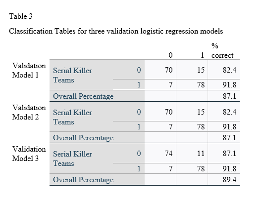
The Nagelkerke R Square for the worst performing validation model was 0.657. The Nagelkerke R Square for the best performing model was 0.706. The mean Nagelkerke R Square was 0.684. The difference in means of the Nagelkerke R Squares for the initial and validation models was 1.8%.
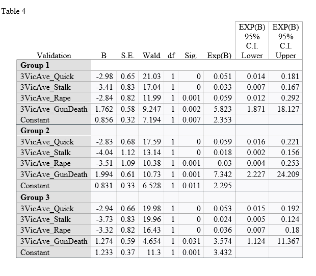
The average binary logistic regression model for the three validation models was found to be Serial Killer Team = 0.973[Constant] + -2.918*Quick Kill + -3.726*Stalking + -3.224*Rape + 1.677*Gun Death, where positive values indicated the act was predicted to be an instance of Serial Killer Teams and negative values indicative of Individual Serial Killers. The range of beta weights for the independent variables and constants were -2.983 to -2.834 for Quick Kill, -4.042 to -3.410 for Stalking, -3.513 to -2.837 for Rape, 1.274 to 1.994 for Gun Death, and 0.831 to 1.233 for the constant. These results, as all lows and highs for all independent variables were of the same sign, support the finding that Serial Killer Teams are more likely to kill by gun and less likely to kill quickly, stalk, or rape, and the opposite was found for Individual Serial Killers, across all validation models and validated the first nine models.
The individual binary logistic regression models for the validation models can be seen in Table 4
CatPCA Models
CatPCA analyses were conducted on the same data of three groupings of 85 random individuals and 85 random teams as the three validation models, as an alternative method of validating the variance accounted for in the binary logistic regressions. All variables used in the previous models were included in the CatPCA analyses, including the Teams-Individual Serial Killer variable that was the dependent variable in the logistic models. All variables were discretized using the “Multiplying” method. There were no missing values in the data in any of the variables used in analyses. The solutions were rotated using the Varimax rotation with Kaiser normalization.
The appropriate number of dimensions was checked by setting the “Dimensions in solution” to three, and then checking to see how many had eigenvalues greater than 1. As
expected, because the, only two dimensions had eigenvalues greater than one, indicating two dimensions would be appropriate for the CatPCA analyses.
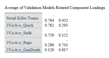
Cronbach’s Alpha for the three models was 0.876, 0.899, and 0.881, respective to the order of analysis, and the Variance Accounted For was 66.934%, 71.216%, and 67.762%, respective to the order of analysis. The mean of the variance accounted for by the three CatPCA models was 68.637%, which was 0.27% different from the mean Naglekerke R Square approximation for explained variance in the three logistic models that used the same samples.
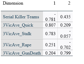
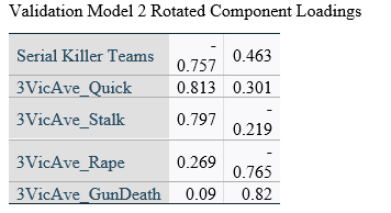
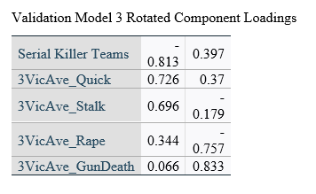
In all three models, variables loaded onto the same dimensions with similar magnitudes and directions.
Object scores for dimension one were almost exclusively negative values if the instance was committed by team killers for all three samples, which would represent a similar finding as the binary logistic regression models, in that teams did not participate in stalking, raping, or quick killing to the same degree individual serial killers did.
The individual rotated component loadings (boxcar) for two dimensions in the CatPCA models can be seen in Table 5.
Table 5
CatPCA Rotated Component Loadings
Validation Model 1 Rotated Component Loadings (Can’t PCA be better displayed graphically? – Short answer is “Yes”, but I do not have graphics and cannot produce any additional at this time)
Alternate Model with Fewer Victims
The research question for this project concerned whether information on three victims would be enough to determine if the acts were committed by teams or individual serial killers. To test whether it may be possible to make such a determination with fewer kills, an alternate binary logistic regression analysis was performed on the Group 1 data, using the dummy variables for Quick Kill, Stalking, Rape, and Gun Death for the first two victims.
The resulting model was specified as Serial Killer Team or Individual = 1.065[Constant] + 1.437 * Victim 1 Gun Death + -3.728*Victim 1 Stalking + -3.228*Victim 1 Rape + -3.028*Victim 2 Quick Kill. Positive values indicated the act was predicted to be an instance of Serial Killer Teams. Negative values were indicative of Individual Serial Killers, just as all logistic regression models in this project that included three victim averages for method of kill, weapon, and victim treatment variables. All independent variables were found to be significant (p<=.001), and the highest correlation between any two independent variables was -0.412 (Victim 1 Gun Death and Victim 2 Quick Kill) meaning collinearity was not an issue.
Discussion
While the results presented in this project are of interest, the data set for all analyses used in this project contained only information on serial killer teams and individuals who committed at least three killings, and there may be substantial differences in serial killers with only two victims. The research question regarding fewer victims may be explored in future projects. Additionally, all analyses looked only at the victim order and not the specific number of murders at points in time; multiple murders in a single time and setting may account for all of a serial killer’s victims used these analyses for some instances. Future analyses will incorporate the timing and settings of murders and number of victims at each instance in time.
The goal of this study was comparative analysis of the variant characteristics of serial killer teams and soloists. A recurring issue in serial killer studies is the lack of reputable, available data 3. Attempting to analyze a subset of serialists compounds the struggle of finding a quality data set. This reinforces the need for a standard monitoring system as suggested by Hodgkinson, et al. 4 and Mouzos, et al. 5. While the results of the current study were not all novel, the means by which the results were obtained does not have a current presence in the literature.
The following four variables were shown to be significant: quick, stalk, rape, and gun death. Teams were less likely to stalk, rape, and be quick in killing their victims but more likely to use a gun. Based on the complete profile created by these results, it is interesting that teams are more likely to use a gun but less likely to complete their murders in a quick manner. In regards to means of deadly force, a gun would seemingly be one of the most time efficient methods for killing. Furthermore, previous research showed that more than 50% of teams used multiple methods to kill a single victim 6.
Another question raised by the “slow” nature of team homicides versus their “quick” solo counterparts is whether this is related to their self-imposed geographic limitations. Hickey noted that teams are more likely to reside close to their killing grounds 7. Are team killers more comfortable taking their time and accumulating more victims because of their proximity to their home base? Is it possible that the added risk of bringing another individual into the equation restricts the geographical comfort zone?
Although previous research identified sexual motivations as being the most common among team killers, the results of this study showed that teams are less likely to rape their victims than solo serial killers. If gratification is not obtained via raping the victim, is it simply the act of killing that gives teams sexual fulfillment? Or is it the witnessing of a kill for a submissive partner or instructing another to kill for a dominant partner?
While the results presented in this project are of interest, the data set for all analyses contained only information on serial killer teams and individuals who committed at least three killings, and there may be substantial differences in serial killers with only two victims. Use of a different database or of the ‘two-victim’ definition of a serial killer may allow for a larger sample that could yield different variables of significance for developing models are two options for future research in comparative analysis of teams and solo serial killers. All analyses looked only at the victim order and not the specific number of murders at points in time; multiple murders in a single time and setting may account for all of a serial killer’s victims used these analyses for some instances. Future analyses will incorporate the timing and settings of murders and number of victims at each instance in time.
References
1. Holmes RM, Holmes ST. Contemporary perspectives on serial murder. Thousand Oaks, CA: Sage Publications; 1998.
2. Woster M. Differences in Characteristics of Criminal Behavior Between Solo and Team Serial Killers and Team Serial Kill [Dissertation]. Digital Commons@NLU: Clinical Psychology, National Louis University; 2020.
3. Luc E. Latent class analysis of serial murderers, The University of North Carolina at Charlotte; 2016.
4. Hodgkinson S, Prins H, Stuart-Bennett J. Monsters, madmen… and myths: A critical review of the serial killing literature. Aggression and violent behavior. 2017;34:282-289.
5. Mouzos J, West D. An examination of serial murder in Australia. Trends & Issues in Crime & Criminal Justice. 2007(346).
6. Walters BK, Drislane LE, Patrick CJ, Hickey E. Serial murder: Facts and misconceptions. Science and the Courts. 2015;1(5):32-41.
7. Hickey EW. Serial murderers and their victims. 7th ed. ed. Boston, MA, USA: Cengage Learning 2016.